


By Renato Rimolo-Donadio, renato.rimolo@rydevinc.com
S-parameters (or scattering parameters) are the most used representation for interconnect models in the frequency domain, whether derived from analytical models, simulations, or measurements. They offer a straightforward representation, with ease of reading, of transmission, reflection, and crosstalk. Additionally, as a form of microwave network parameters, they can be combined with standard matrix algebra; the matrices are well-behaved, exhibiting a good condition number because the magnitude of the entries fall within the range of 0 to 1 for passive interconnects.
A S-Parameter block defines the port terminal relations of a linear system in terms of the incident (a) and reflected waves (b) at each port, normalized to a reference impedance, typically 50 Ohm. The matrix entries define the relationship between different ports, reflection for input ports, transmission for intentionally connected ports, or crosstalk for electromagnetic coupling, as depicted in Fig. 1.
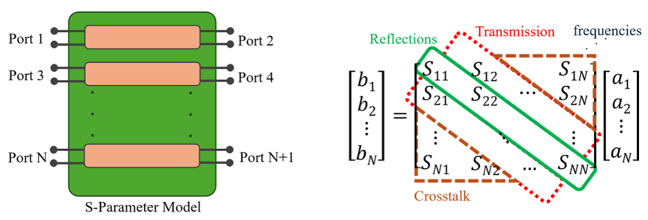
It is crucial that each port is situated where a unique voltage and current can be defined, in such a way that the field quantities can be translated to circuit quantities, voltage and current, to properly represent the interface behavior. A good reference to microwave network parameters is Pozar’s Microwave Engineering book [1]
All signal integrity tools or measurement software are capable of handling S-parameters, but it is often the case that the files come from different sources, with different bandwidth, resolutions, or port order; Consequently, data manipulation is frequently necessary before comparisons or further model concatenation can occur. This ensures the generation of standardized parameters that can be conveniently interpreted and visualized.
In this first blog post, we will review how to easily manage S-Parameter files in Matlab [2], using functions from its RF Toolbox [3]. We will use as an example, the cases in the reference [4], which were generated with a semi-analytical solver developed by TET-TUHH [5]. This solver utilizes physics-based via and trace models conceived for multilayer substrates, described in the reference [6].
The example we will use represents a simplified backplane interconnect model from [6], depicted in Fig. 2. This model features three single-ended links running in parallel across two cards and a backplane, using a different number of return vias in close proximity to the signal vias, with 1, 2 and 4 ground vias, as the filename indicates.
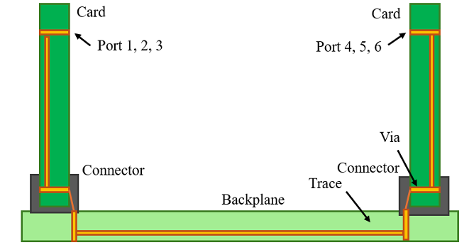
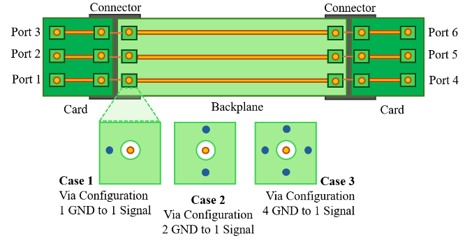
Figure 2. Backplane simplified case used as example, adapted from [4]: a) Cross-section diagram, and b), connectivity diagram. Touchstone files preserve the same port convention, with the same via GND/Signal ratio for all vias in each of the three cases.
The Touchstone format in its first version uses the .sNp extension, where the N refers to the number of ports. Version two of the format recommends substituting this extension, which has a potential variable length, with the extension .ts. The initial version of the Touchstone format uses the .sNp file extension, where ‘N’ denotes the number of ports. In version 2, the format suggests replacing this potentially variable-length extension with .ts. However, version 1 remains widely used due to its simplicity, despite the additional features offered in version 2. The complete specifications for both versions 1 and 2 can be downloaded from the IBIS forum webpage [7].
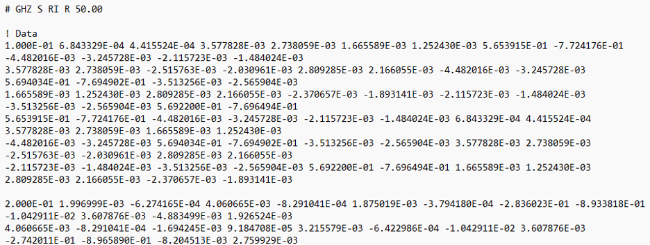
The format itself is quite straightforward. It begins with the header line that specifies the units of the frequency vector, the type of microwave network parameter (S-parameters in this case), the data format (typically Real-Imaginary), and the normalization impedance (commonly 50 Ohms). Following the header, each entry consists of a frequency point, immediately followed by the real and imaginary parts of the matrix entries corresponding to that frequency; this pattern continues for all subsequent frequency points. An illustrative example of the beginning of such a file is provided in Fig. 3.
To begin, we can import these three files into Matlab using the sparameters function.
path= "[location of the files]";
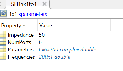
SELink1to1 = sparameters(strcat(path,"backplane_3SElinks_1to1_20G.s6p"))
SELink2to1 = sparameters(strcat(path,"backplane_3SElinks_2to1_20G.s6p"))
SELink4to1 = sparameters(strcat(path,"backplane_3SElinks_4to1_20G.s6p"))
This function creates an S-parameter handler, with a specific structure. It includes two numerical variables: one for the normalization impedance (Impedance) and another for the number of ports defined in the imported file (NumPorts). Additionally, it contains a three-dimensional matrix of size n × n × number of frequencies (Parameters), with the frequency vector itself (Frequencies).
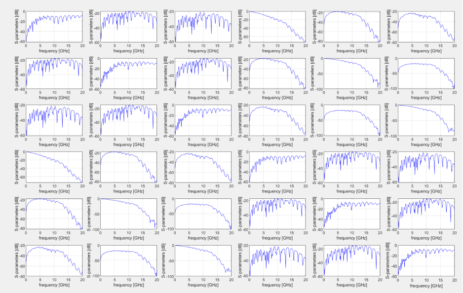
Now that the data for all three cases is loaded into our workspace, we have the flexibility to manipulate it as needed. One useful plot for understanding the contents of an S-parameter structure is a comprehensive matrix overview. This helps in identifying the relationships between ports as defined in the Touchstone file, and it could be generated through this simple function for the magnitude of the S-parameters, which sweeps the matrix entries across the frequency vector within an n x n subplot (Fig. 4).
					plot_parameters_mag(SELink1to1.Parameters, SELink1to1.Frequencies, 'b');

% function for overview plot
function plot_parameters_mag(Matrix,freq,color)
    figure
    [porti,portj,Nfreqs]=size(Matrix);
    counter=1;
        for n=1:porti
            for m=1:portj
                set(gca,'FontSize',8);
                subplot(porti,portj,counter);
                temporalVector=squeeze(Matrix(n,m,:));
                plot(freq./1e9,20*log10(abs(temporalVector)),'Color',color);
                hold on;
                grid on;
                xlabel('frequency [GHz]');
                ylabel('S-parameters [dB]');
                counter=1+counter;
            end
        end
end
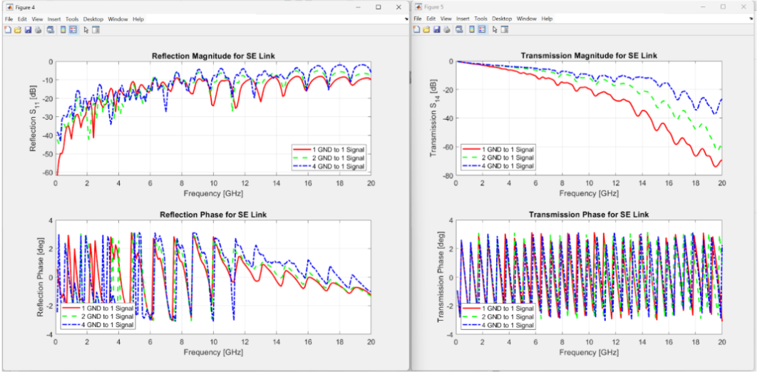
It is frequently necessary to create professional-looking plots for specific S-parameter data across various datasets. For example, to visualize the magnitude and phase of reflection (S11) and transmission and transmission (S14) for our sample cases, magnitude and phase, we can arrange them within a 2×1 subplot. With some additional commands, the plots can be tailored to the three S-parameter structures we previously imported.
The code provided next will generate the two editable plot windows shown in Fig. 5. There, we can reproduce the plots from reference [4] showcasing the simulated responses found in the .s6p files for different via return path configurations.
					%plot reflection at port 1
Fig1 = figure
Fig1a = subplot(2,1,1); %create subplot 1
hold on
grid on
box(Fig1a,'on')
set(gca,'FontSize',12);
plot(Fig1a, SELink1to1.Frequencies/1e9, 20*log10(squeeze(abs(SELink1to1.Parameters(1,1,:)))), 'Color', 'r', 'LineWidth', 2);
plot(Fig1a, SELink2to1.Frequencies/1e9, 20*log10(squeeze(abs(SELink2to1.Parameters(1,1,:)))), 'Color', 'g', 'LineWidth', 2, 'LineStyle', '--');
plot(Fig1a, SELink4to1.Frequencies/1e9, 20*log10(squeeze(abs(SELink4to1.Parameters(1,1,:)))), 'Color', 'b', 'LineWidth', 2, 'LineStyle','-.');
xlabel(Fig1a, "Frequency [GHz]")
ylabel(Fig1a, "Reflection S_{11} [dB]")
legend("1 GND to 1 Signal", "2 GND to 1 Signal", "4 GND to 1 Signal")
legend('Location','southeast')
title("Reflection Magnitude for SE Link")
Fig1b = subplot(2,1,2); %create subplot 2
hold on
grid on
box(Fig1b,'on')
set(gca,'FontSize',12);
plot(Fig1b, SELink1to1.Frequencies/1e9, (squeeze(angle(SELink1to1.Parameters(1,1,:)))), 'Color', 'r', 'LineWidth', 2);
plot(Fig1b, SELink2to1.Frequencies/1e9, (squeeze(angle(SELink2to1.Parameters(1,1,:)))), 'Color', 'g', 'LineWidth', 2, 'LineStyle', '--');
plot(Fig1b, SELink4to1.Frequencies/1e9, (squeeze(angle(SELink4to1.Parameters(1,1,:)))), 'Color', 'b', 'LineWidth', 2, 'LineStyle','-.');
xlabel(Fig1b, "Frequency [GHz]")
ylabel(Fig1b, "Reflection Phase [deg]")
legend("1 GND to 1 Signal", "2 GND to 1 Signal", "4 GND to 1 Signal")
legend('Location','southwest')
title("Reflection Phase for SE Link")

% plot transmission between ports 1 and 4
Fig2 = figure
Fig2a = subplot(2,1,1); %create subplot 1
hold on
grid on
box(Fig1a,'on')
set(gca,'FontSize',12);
plot(Fig2a, SELink1to1.Frequencies/1e9, 20*log10(squeeze(abs(SELink1to1.Parameters(1,4,:)))), 'Color', 'r', 'LineWidth', 2);
plot(Fig2a, SELink2to1.Frequencies/1e9, 20*log10(squeeze(abs(SELink2to1.Parameters(1,4,:)))), 'Color', 'g', 'LineWidth', 2, 'LineStyle', '--');
plot(Fig2a, SELink4to1.Frequencies/1e9, 20*log10(squeeze(abs(SELink4to1.Parameters(1,4,:)))), 'Color', 'b', 'LineWidth', 2, 'LineStyle','-.');
xlabel(Fig2a, "Frequency [GHz]")
ylabel(Fig2a, "Transmission S_{14} [dB]")
legend("1 GND to 1 Signal", "2 GND to 1 Signal", "4 GND to 1 Signal")
legend('Location','southwest')
title("Transmission Magnitude for SE Link")
Fig2b = subplot(2,1,2); %create subplot 2
hold on
grid on
box(Fig2b,'on')
set(gca,'FontSize',12);
plot(Fig2b, SELink1to1.Frequencies/1e9, (squeeze(angle(SELink1to1.Parameters(1,4,:)))), 'Color', 'r', 'LineWidth', 2);
plot(Fig2b, SELink2to1.Frequencies/1e9, (squeeze(angle(SELink2to1.Parameters(1,4,:)))), 'Color', 'g', 'LineWidth', 2, 'LineStyle', '--');
plot(Fig2b, SELink4to1.Frequencies/1e9, (squeeze(angle(SELink4to1.Parameters(1,4,:)))), 'Color', 'b', 'LineWidth', 2, 'LineStyle','-.');
xlabel(Fig2b, "Frequency [GHz]")
ylabel(Fig2b, "Transmission Phase [deg]")
legend("1 GND to 1 Signal", "2 GND to 1 Signal", "4 GND to 1 Signal")
legend('Location','southwest')
title("Transmission Phase for SE Link")
Once you have processed, manipulated, or resampled the S-parameters, you can easily export them back in Touchstone file format using Matlab’s rfwrite function.
rfwrite(SELink1to1,srcat(path, "SELink1to1_modified.s6p"));
You no longer have to rely on screenshots or rough visual comparisons between different figures in your reports, presentations, or papers! Instead, you can generate precise, integrated, and professional-looking plots directly using a few lines of Matlab code
If you are interested in learning more about this topic, or would like to know more about Rydev, contact us: info@rydevinc.com
References:
[1] David M. Pozar, Microwave engineering, 4th ed. Chapter 4. Wiley, 2012. ISBN 978-0-470-63155-3
[2] Mathworks. Matlab, [available online]: https://www.mathworks.com/
[3] Mathworks, Matlab RF Toolbox, [available online]: https://www.mathworks.com/products/rftoolbox.html
[4] R. Rimolo-Donadio, T.-M. Winkel, C. Siviero, D. Kaller, H. Harrer, H.-D. Brüns, and C. Schuster. “Fast Parametric Pre-Layout Analysis of Signal Integrity for Backplane Interconnects,” in Proc. 15th IEEE 15th IEEE Workshop on Signal Propagation on Interconnects (SPI), Naples, Italy, May 2011. 10.1109/SPI.2011.5898839
[5] Institut fuer Theoretische Elektrotechnik, Technische Universitaet Hamburg (TUHH), CONCEPT EM Software: CONMLS, Multilayer Substrate Simulator, [documentation available online]: https://www.tet.tuhh.de/wordpress/wp-content/uploads/2024/07/Manual-Conmls.pdf
[6] R. Rimolo-Donadio, X. Gu, Y. H. Kwark, M. B. Ritter, B. Archambeault, F. De Paulis, Y. Zhang, J. Fan, H.-D. Brüns, and C. Schuster. “Physics-Based Via and Trace Models for Efficient Link Simulation on Multilayer Structures up to 40 GHz,” IEEE Transactions on Microwave Theory and Technologies, vol. 57, no. 8, Aug. 2009. 10.1109/TMTT.2009.2025470
[7] IBIS Open Forum: https://ibis.org/ Touchstone® File Format Specification, version 2.1, [available online]: https://ibis.org/touchstone_ver2.1/touchstone_ver2_1.pdf, and version 1.1, [available online]: https://ibis.org/connector/touchstone_spec11.pdf